Udacity’s Sensor Fusion Nanodegree Program!

Udacity’s Sensor Fusion Nanodegree Program launched yesterday! I am so happy to get this one out to students 😁

Goal

The goal of this program is to offer a much deeper dive into perception and sensor fusion than we were able to do in our core Self-Driving Car Engineer Nanodegree Program. This is a great option for students who want to develop super-advanced, cutting-edge skills for working with lidar, camera, and radar data, and fusing that data together.

The first three months of the program are brand new content and projects that we’ve never taught before. The final month, on Kalman filters, comes from our core Self-Driving Car Nanodegree Program. The course is designed to last four months for new students. Students who have already graduated the core Self-Driving Car Engineer Nanodegree Program should be able to finish this specialized Sensor Fusion Nanodegree Program in about three months.

Curriculum

Course 1: Lidar
Instructor: Aaron Brown, Mercedes-Benz
Lesson: Introduction. View lidar point clouds with Point Cloud Library (PCL).
Lesson: Point Cloud Segmentation. Program the RANSAC algorithm to segment and remove the ground plane from a lidar point cloud.
Lesson: Clustering. Draw bounding boxes around objects (e.g. vehicles and pedestrians) by grouping points with Euclidean clustering and k-d trees.
Lesson: Real Point Cloud Data. Apply segmentation and clustering to data streaming from a lidar sensor on a real self-driving car.
Lesson: Lidar Obstacle Detection Project. Filter, segment, and cluster real lidar point cloud data to detect vehicles and other objects!

Course 2: Radar
Instructor: Abdullah Zaidi, Metawave
Lesson: Radar Principles. Measure an object’s range using the physical properties of radar.
Lesson: Range-Doppler Estimation. Perform a fast Fourier transform (FFT) on a frequency modulation continuous wave (FMCW) radar signal to create a Doppler map for object detection and velocity measurement.
Lesson: Clutter, CFAR, AoA. Filter noisy radar data in order to reduce both false positives and false negatives.
Lesson: Clustering and Tracking. Track a vehicle with the Automated Driving System Toolbox in MATLAB.
Lesson: Radar Target Generation and Detection Project. Design a radar system using FMCW, signal processing, FFT, and CFAR!

Course 3: Camera
Instructor: Andreas Haja, HAJA Consulting
Lesson: Computer Vision. Learn how cameras capture light to form images.
Lesson: Collision Detection. Design a system to measure the time to collision (TTC) with both lidar and camera sensors.
Lesson: Tracking Image Features. Identify key points in an image and track those points across successive images, using BRISK and SIFT, in order to measure velocity.
Project: 2D Feature Tracking. Compare key point detectors to track objects across images!
Lesson: Combining Camera and Lidar. Project lidar points backward onto a camera image in order to fuse sensor modalities. Perform neural network inference on the fused data in order to track a vehicle.
Lesson: Track An Object in 3D. Combine point cloud data, computer vision, and deep learning to track a moving vehicle and estimate time to collision!

Course 4: Kalman Filters
Instructors:
Dominic Nuss, Michael Maile, and Andrei Vatavu, Mercedes-Benz
Lesson: Sensors. Differentiate sensor modalities based on their strengths and weaknesses.
Lesson: Kalman Filters. Combine multiple sensor measurements using Kalman filters — a probabilistic tool for data fusion.
Lesson: Extended Kalman Filters. Build a Kalman filter pipeline that smoothes non-linear sensor measurements.
Lesson: Unscented Kalman Filters. Linearize data around multiple sigma points in order to fuse highly non-linear data.
Project: Tracking with an Unscented Kalman Filter. Track an object using both radar and lidar data, fused with an unscented Kalman filter!

Partners

One of the highlights of working at Udacity is partnering with world experts to teach complex skills to anybody in the world.

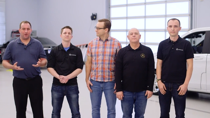
In this program we are fortunate to work especially closely with autonomous vehicle engineers from Mercedes-Benz. They appear throughout the Nanodegree Program, often as the primary instructors, and sometimes simply offering their expertise and context on any other topic.

MathWorks has also proven terrific partners by offering our students free educational licenses for MATLAB. The radar course in this program is taught primarily in MATLAB and leverages several of their newest and most advanced toolboxes.

Reflection

There is a quote, from a completely different context, “It took forever and then it took a night.”

That sums up how I felt building this Nanodegree Program. We spent over a year kicking around ideas for this program, starting work and stopping work, and there were times I thought it wasn’t going to happen. Then we got the right group of instructors together it came together faster than I ever imagined, and it’s beautiful.

Heaven, Hell, and Markov Decision Processes

I’ve been thumbing through Sebastian’s magnum opus, Probabilistic Robotics. The book is now 13 years old, but it remains a great resource for roboticists. Kind of funny to think that, when Sebastian wrote this, he hadn’t even started to work on self-driving cars yet!

The chapter on Markov decision processes (MDPs) covers how to make robotic planning decisions under uncertainty. One of the key assumptions of MDPs is that the agent (robot) can observe its environment perfectly. This turns out to be an unrealistic assumption, which leads to further types of planning algorithms, principally partially observable Markov decision processes (POMDPs).

Nonetheless, ordinary Markov decision processes are a helpful place to start when thinking about motion planning.

I love the exercises at the end of each chapter of Probabilistic Robotics. There is a fun one called “Heaven or Hell” at the end of the MDP chapter. This is actually a variation on a toy problem long-used in the field of motion planning.

Heaven or Hell?

“In this exercise, you are asked to extend dynamic programming to an environment with a single hidden state variable. The environment is a maze with a designated start marked “S”, and two possible goal states, both marked “H”.

“What the agent does not know is which of the two goal states provides a positive reward. One will give +100, whereas the other will give -100. There is a .5 probability that either of those situations is true. The cost of moving is -1; the agent can only move into the four directions north, south, east, and west. Once a state labeled “H” has been reached, the play is over.”

So far, so good.

“(a) Implement a value iteration algorithm for this scenario. Have your implementation compute the value of the starting state. What is the optimal policy?”

The optimal policy here depends on whether we assume the agent must move. If the agent is allowed to remain stationary, then the value of the starting state is 0, because the optimal policy is to stay put.

Calculating the expected reward from reaching state “H” is straightforward. The expected reward is 0, because there’s a 50% chance of a +100 reward, but also a 50% chance of a -100 reward.

0.5 * (+100) + 0.5 * (-100) = 50 + (-50) = 0

Once we establish that, the optimal policy is intuitive. There is no positive reward for reaching any state, but there is a cost to moving to any state. Don’t incur a cost if there’s no possible reward.

The optimal policy changes, however, if the rules state that we must move. In that case, we want to end the game as quickly as possible.

Under this set of rules, the value function decreases as we approach either “H”. The intuition is that the game has no benefits, only costs, so we want to end the game as quickly as possible. From a policy perspective, we want to follow the gradient toward higher values, so if we start at “S”, we wind up trending toward “H”.

“(b) Modify your value algorithm to accommodate a probabilistic motion model: with 0.9 chance the agent moves as desired; with 0.1 chance it will select any of the other three directions at random. Run your value iteration algorithm again, and compute both the value of the starting state, and the optimal policy.”

Once again, the optimal policy depends on whether we can remain stationary. If we can remain stationary, then the value of all cells is 0, and the optimal policy is to stay put. The uncertainty in motion that has just been introduced does not affect the policy, because there’s still no reward for moving anywhere.

If, however, we are required to move, calculating the policy becomes more complex. At this point we really need a computer to calculate the value function, because we have to iterate over all the cells on the map until values converge. For each cell, we have to look at each action and sum the 90% probability that the action will execute properly, and the 10% probability that the action will misfire randomly. Then we pick the highest-value action. Once we do this for every cell, we repeat the cycle over all the cells again, and we keep doing this until the values stabilize.

The first pass in the iteration sets all cells to 0. Depending on which direction we iterate from, the next step might look like this:

Nonetheless, even without a computer, it seems pretty clear that the optimal policy is still for our agent to stay put in the start cell. Without any information about which “H” is heaven and which is hell, there’s no ultimate reward for going anywhere.

“(c) Now suppose the location labeled X contains a sign that informs the agent of the correct assignment of rewards to the two states labeled “H”. How does this affect optimal policy?”

Without computing the policy, it seems likely that the optimal policy will involve going to the sign, identifying heaven and hell on the map, and then proceeding to heaven.

This policy seems qualitatively clear because of the relatively high payoff for reaching heaven (+100), the relatively low cost of motion (-1), the relatively high probability of the motion executing accurately (0.9), and the relatively small size of the map (distance from S to X to H = 19).

It’s easy to imagine tweaking these parameters such that it’s no longer so obvious that it makes sense to go find the sign. With different parameters, it might still make sense to stay put at S.

“(d) How can you modify your value iteration algorithm to find the optimal policy? Be concise. State any modifications to the space over which the value function is defined.”

Basically, we need to figure out the value of reaching the sign. There are essentially two value functions: the value function when we cannot observe the state, and the value function when we can.

Another way to put this is that going to the sign is like taking a measurement with a sensor. We have prior beliefs about the state of the world before we reach the sign, and then posterior beliefs once we get the information from the sign. Once we transition from prior to posterior beliefs, we will need to recalculate our value function.

An important point here is that this game assumes the sign is 100% certain, which makes the model fully observable. That’s not the case with normal sensors, which is why real robots have to deal with partially observable Markov decision processes (POMDPs).

“(e) Implement your modification, and compute both the value of the starting state and the optimal policy.”

Again, we’d need to write code to actually implement this, but the general idea is to have two value functions. The value of X will be dependent on the posterior value function (the value function that we can calculate once we know which is heaven and which is hell). Then we use that value of X to calculate our prior distribution.

For example, here are the value functions, assuming perfect motion:

The posterior value function, after reading the sign at “X”.
The prior value function, before reading the sign at “X”.

Waymo Opens To The Public

Last week, Waymo announced it will put 10 of its vehicles on Lyft’s network in Phoenix. Any Lyft user will be able to ride.

This is super-duper exciting! Waymo is several years ahead of everybody else developing self-driving cars, but until now their vehicles have been off-limits to the general public. I see them scooting around Mountain View all the time, but the only way I can get a ride in one is to pull a favor from a friend who works there.

Now Waymos will be open, albeit in very small initial numbers, to anybody in Phoenix, via Lyft’s network.

This announcement also makes Phoenix the second place in the world, alongside Lyft’s partnership with Aptiv in Las Vegas, where a member of the general public can hail a self-driving robotaxi. They still come with safety drivers, but it’s nonetheless a big step forward.

Literature Review: Capsule Networks

My Udacity colleague, Cezanne Camacho, is preparing a presentation on capsule networks and gave a draft version in the office today. Cezanne is a terrific engineer and teacher, and she’s already written a great blog post on capsule networks, and she graciously allowed me to share some of that here.

Capsule networks come from a 2017 paper by Sara Sabour, Nicholas Frosst, and Geoffrey Hinton at Google: “Dynamic Routing Between Capsules”. Hinton, in particular, is one of the world’s foremost authorities on neural networks.

As my colleague, Cezanne, writes on her blog:

Capsule Networks provide a way to detect parts of objects in an image and represent spatial relationships between those parts. This means that capsule networks are able to recognize the same object in a variety of different poses even if they have not seen that pose in training data.

Love the Pacman GIF. Did I mention Cezanne is also an artist?

Cezanne explains that a “capsule” encompasses features that make up a piece of an image. Think of an image of a face, for example, and imagine capsules that capture each eye, and the nose, and the mouth.

These capsules organize into a tree structure. Larger structures, like a face, would be parent nodes in the tree, and smaller structures would be child nodes.

“In the example below, you can see how the parts of a face (eyes, nose, mouth, etc.) might be recognized in leaf nodes and then combined to form a more complete face part in parent nodes.”

“Dynamic routing” plays a role in capsule networks:

“Dynamic routing is a process for finding the best connections between the output of one capsule and the inputs of the next layer of capsules. It allows capsules to communicate with each other and determine how data moves through them, according to real-time changes in the network inputs and outputs!”

Dynamic routing is ultimately implemented via an iterative routing process that Cezanne does a really nice job describing, along with the accompanying math, in her blog post.

Capsule networks seem to do well with image classification on a few datasets, but they haven’t been widely deployed yet because they are slow to train.

In case you’d like to play with capsule networks yourself, Cezanne also published a Jupyter notebook with her PyTorch implementation of the Sabour, Frosst, and Hinton paper!

NXP Earnings And The Future Of Automotive Manufacturing

I spent a few hours this morning racing down the rabbit hole of NXP’s Q1 2019 earnings call, which I wrote up for Forbes.com:

“The transcript highlights, in particular, the distinction between NXP’s traditional automotive semiconductor business, which declined, and its advanced driver assistance systems (ADAS) and battery management systems (BMS), both of which grew dramatically, albeit from small bases.”

NXP is kind of like the automotive industry in miniature: vehicle sales are declining today, causing decreases in revenue associated with traditional automotive manufacturing. But in the not-so-distant future, mobility will change and new products, like advanced driver assistance systems and battery management systems, will grow quickly.

Read the whole thing.

And I should also mention that my Forbes.com editor, Alan Ohnsman, has recruited a terrific stable of automotive writers. The daily output of the Forbes.com transportation section is voluminous. Just in the last day you can read about shadow testing at Tesla, Ford’s Q1 earnings, the effect of self-driving cars on the automotive repair market, Ford’s connected vehicles efforts, GM’s upcoming electric pickup truck, Tesla’s cash crunch, Ford’s investment in Rivian, and Waymo’s lidar units.

Self-Driving Car Ethics

My Udacity colleague Vienna Harvey sat down with Australian podcaster Zoe Eather to discuss the role of both ethics and education as they relate to self-driving cars. It’s a fun episode 🙂

This interview is part of Zoe’s Smart Community podcast, which covers everything from infrastructure, to data, to climate change, to mobility.

Prior to Vienna’s interview, I got to take Zoe for a spin in Carla, Udacity’s self-driving car. Zoe was delightful and I think you’ll enjoy listening to her and Vienna geek out about self-driving cars.

AI Robotic Racing

Lockheed Martin, NVIDIA, and the Drone Racing League have partnered to create AIRR: Artificial Intelligence Robotic Racing.

The gist seems to be that the top team to build an autonomous racing drone will win $1 million, and there is an addition $250,000 available to whoever can first beat a human drone pilot in a race.

I had not known about the Drone Racing League, but the videos look pretty cool.

As a person without much hand-eye coordination, it kind of blows my mind that pilots can navigate these types of environments.

On the other hand, as a person with limited hand-eye coordination, it seems like computers would be much better at this than me. Maybe than everybody?

Bjarne Stroustrup on 40 of C++

Recently I sat down with Bjarne Stroustrup, the creator of C++, to discuss his career and the evolution of C++ over years.

We discussed Bjarne’s origins in Denmark, his PhD work at Cambridge, the origins of C++ at Bell Labs, how to teach C++, the ISO committee that governs C++, and what exactly made Bjarne’s career so successful. There’s a lot more, too 😀

Watch the interview here.

And if you are interested in learning C++ from Bjarne (and me, and many other instructors), enroll in Udacity’s C++ Nanodegree Program!