Ford plays catch up on self-driving car technology. No, wait, another article says Ford is ahead! The truth is Ford itself doesn’t really know for sure, because none of the car companies are releasing metrics in this area. The only group that even has a clue about this, interestingly enough, are the automotive suppliers, since they see what everyone is doing.
I thought I’d try to summarize it, mostly as an exercise in trying to understand the paper myself.
Background
This paper appears to originate out of the lab of Raquel Urtasun, the University of Toronto professor who just joined Uber ATG. Prior to Uber, Urtasun compiled the KITTI benchmark dataset.
Right now, MultiNet sits at 15th place on the leaderboard, but it’s the top entry that’s been formally written up in an academic paper.
Goals
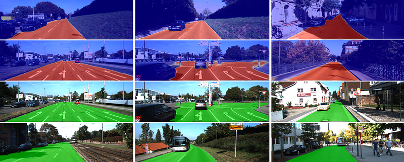
Interestingly, the goal of MultiNet is exactly to win the KITTI Lane Detection competition. Rather, it’s to train a network that can segment the road quickly, in real-time. Adding complexity, the network also detects and classifies vehicles on the road.
¿Por qué no?
Architecture
The MultiNet architecture is three-headed. The beginning of the network is just VGG16, without the three fully connected layers at the end. This part of the network is the “encoder” part of the standard encoder-decoder architecture.
Conceptually, the “CNN Encoder” reduces each input image down to a set of features. Specifically, 512 features, since the output tensor (“Encoded Features”) of the encoder is 39x12x512.
For each region of an input image, this Encoded Features tensor captures a measure of how strongly each of 512 features is represented in that region.
Since this is a neural network, we don’t really know what these features are, and they may not even really be things we can explain. It’s just whatever things the network learns to be important.
The three-headed outputs are more complex.
Classification: Actually, I just lied. This output head is pretty straightforward. The network applies a 1×1 convolution to the encoded features (I’m not totally sure why), then adds a fully connected layer and a softmax function. Easy.
(Update: Several commenters have added helpful explanations of 1×1 convolutional layers. My uncertainty was actually more about why MultiNet adds a 1×1 convolutional layer in this precise place. After chewing on it, though, I think I understand. Basically, the precise features encoded by the encoder sub-network may not be the best match for classification. Instead, the classification output perform best if the shared features are used to build a new set of features that is specifically tuned for classification. The 1×1 convolutional layer transforms the common encoded features into that new set of features specific to classification.)
Detection: This output head is complicated. They say it’s inspired by Yolo and Faster-RCNN, and involves a series of 1×1 convolutions that output a tensor that has bounding box coordinates.
Remember, however, the encoded features only have dimensions 39×12, while the original input image is a whopping 1248×384. Apparently 39×12 winds up being too small to produce accurate bounding boxes. So the network has “rezoom layers” that combine the first pass at bounding boxes with some of the less down-sampled VGG convolutional outputs.
The result is more accurate bounding boxes, but I can’t really say I understand how this works, at least on a first readthrough.
Segmentation: The segmentation output head applies fully-convolutional upsampling layers to blow up the encoded features from 39x12x512 back to the original image size of 1248x312x2.
The “2” at the end is because this head actually outputs a mask, not the original image. The mask is binary and just marks each pixel in the image as “road” or “not road”. This is actually how the network is scored for the KITTI leaderboard.
Training
The paper includes a detailed discussion of loss function and training. The main point that jumped out at me is that there are only 289 training images in the KITTI lane detection training set. So the network is basically relying on transfer learning from VGG.
It’s pretty amazing that any network can score at levels of 90%+ road accuracy, given a training set of only 289 images.
I’m also surprised that the 200,000 training steps don’t result in severe overfitting.
Summary
MultiNet seems like a really neat network, in that it accomplishes several tasks at once, really fast. The writeup is also pretty easy follow, so kudos to them for that.
If you’re so inclined, it might worth downloading the KITTI dataset and trying out some of this on your own.
I’ve got a few trips planned and I hope to meet current and prospective Udacity Self-Driving Car students along the way.
If you’re neither a current nor a prospective student, but would like to meet for another reason, just send me an email (david.silver@udacity.com).
Japan
It looks like a gathering of Udacity Self-Driving Car students in Tokyo will be happening on Wednesday, May 31, at EGG. More details to come in the #japan channel of the student Slack community, or ping me directly for details.
Washington, DC
I’m heading home to Virginia from June 7th through 11th. Still working on organizing a gathering while I’m there. Send me an email if you’re interested in attending.
Denver
I’ll be in Colorado for a week from late June to early July, and Autonomous Denver has graciously offered to help put an event together. More details to come on this, as well. If you’re interested, join the Autonomous Denver Meetup group, or send me an email directly.
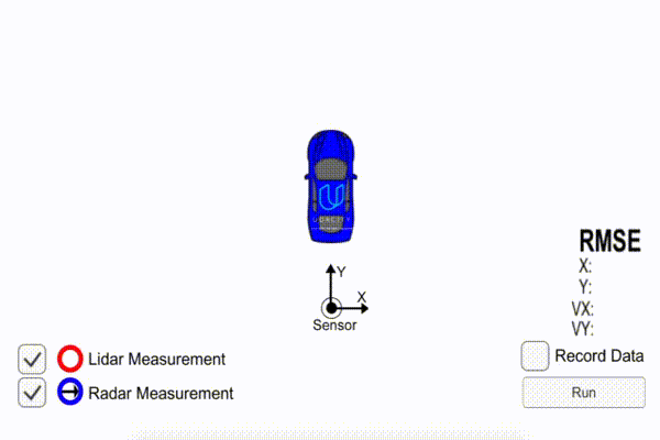
Here is a collection of Udacity student posts, all about Kalman filters. Kalman filters are a tool that sensor fusion engineers use for self-driving cars.
Imagine you have a radar sensor that tells you another vehicle is 15 meters away, and a laser sensor that says the vehicle is 20 meters away. How do you reconcile those sensor measurements?
Jeremy has a really nice post on the intuition behind Kalman filters — why we use them and how they work. Plus the GIF is cool:
“It’s just a cycle of predict (“based on your previous motion, I’d expect you to be here n seconds later”) and measurement update (“but my sensor thinks you’re here”), from which a compromise is made and a new state vector and covariance matrix are determined”
Actually, this quick post is as much about the deep neural networks Andrew experimented with between terms as it is about the Kalman filters from the beginning of Term 2. But he does highlight using behavior driven development to build his Kalman filter pipeline, which is awesome:
“I added Behaviour Driven Development (BDD) tests using Catch to my project. While this took extra time to setup, I’ve seen the benefit of developer tests too many times to ignore them, especially when using verbose languages like C++.”
This post by Mithi is a great place to look if you’re interested in the math behind all of the vectors and matrices that drive the Extended Kalman Filter.
“A lidar can measure distance of a nearby objects that can easily be converted to cartesian coordinates (px, py) . A radar sensor can measure speed within its line of sight (drho)using something called a doppler effect. It can also measure distance of nearby objects that can easily be converted to polar coordinates (rho, phi) but in a lower resolution than lidar.”
Alena’s breakdown of the differences between Kalman Filters, Extended Kalman Filters, and Unscented Kalman Filters is terrific. Here’s the summary, but there’s a lot more at the link:
“In a case of nonlinear transformation EKF gives good results, and for highly nonlinear transformation it is better to use UKF.”
Joshua’s post takes the Kalman filter from the highest-level intuitions, through the mathematical theory, all the way to the algorithmic implementation.
“Kalman filter algorithm can be roughly organised under the following steps: 1. We make a prediction of a state, based on some previous values and model. 2. We obtain the measurement of that state, from sensor. 3. We update our prediction, based on our errors 4. Repeat.”
Testing is one of many open challenges in autonomous vehicle development. There’s no clear consensus on exactly how much testing needs to be done, and how to do it, and how safe is safe enough.
Ding Zhao and Huei Peng, from Michigan, claim to have found a way to reduce by 99.9% the billion-plus miles necessary. The four keys are:
Naturalistic Field Operational Tests
Test Matrix
Worst Case Scenario
Monte Carlo Simulation
The paper is light on details, but the approach seems to boil down to: drive dangerous situations again and again on a test track, instead of waiting for the dangerous situations to occur on the road, because that could take forever.
And that all seems smart enough. It’s like practicing three point shots, instead of just mid-range jumpers. Or building new exciting software projects as a way to learn a new computer language, instead of just maintaining legacy code.
But it’s less clear how to get from essentially “focused practice” to “the car is safe enough”. Perhaps another paper is forthcoming that makes that leap.
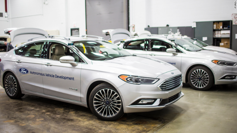
Yesterday, Ford parted ways with CEO Mark Fields, and promoted Jim Hackett to the top spot.
Hackett is an interesting person for a lot of reasons. One reason is Hackett’s one year run as head of Ford Smart Mobility, LLC, immediately prior to now.
The LLC is more of a small standalone business unit, whereas Ford’s autonomous vehicle team, headed by Randy Visintainer, is housed within Ford Motor Company proper.
This distinction raises the question of which is the key market — self-driving cars, or mobility as a service?
Traditional mobility has been delineated by different companies owning different modes of transportation — the railway company is different than the car company, which is different than the bike or bus company.
Will technology change that in the future? Or is the future pretty much about self-driving taxis, with people using bikes and trains and planes more or less as they always have?
I’m not quite sure. Certainly, as people give up their personal cars and rely on ridesharing, there perspective on other forms of transportation changes. If your self-driving taxi company can’t take you 200 miles to your weekend getaway, and you don’t have your own car, maybe you need a seamless solution. Or maybe you just call Hertz.
It’s not obvious that Ford or Hackett will bank on broad mobility over pure self-driving cars, but it seems like a possibility.
Maybe this is all just about profit margins and exiting underperforming markets to focus on stronger ones. Ford is reducing 10% of its workforce, for similar reasons.
But it’s also easy to imagine these are early steps in a longer-term disruption of the automotive industry — a change from automotive sales to mobility.
To be sure, consumer automotive sales will continue for a long time, especially in rural areas. But the bright future of automotive manufacturers probably lies in fleet sales to ride sharing companies, or maybe even becoming ride sharing companies themselves. Pulling back from foreign markets might be part of that trend.