They confess that a few years ago, their development process was slow:
“Our first production models were taking days to train due to increases in data and model sizes.…Our initial deployment process was complex and model developers had to jump through many hoops to turn a trained model into a “AV-ready” deployable model….We saw from low GPU and CPU utilization that our initial training framework wasn’t able to completely utilize the hardware.”
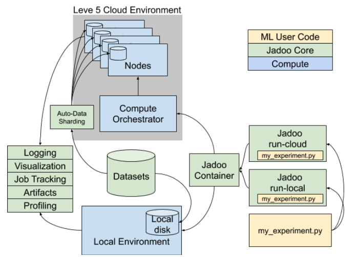
The post proceeds to described the new pipeline Lyft built to overcome these obstacles. They started with a proof-of-concept for lidar point cloud segmentation, and then grew that into a production system.
The pipeline accomplishes a lot of infrastructure wins.
Testing. The pipeline incorporates continuous integration testing, both to ensure that the models don’t regress, and also to verify that the code researchers write will run in the PyTorch-based vehicle environment.
Containerization. Lyft invested in a uniform container environment, to mitigate the distinction between local and cloud model training.
Deployment. The system relies heavily on LibTorch and TorchScript for deployment to the vehicle’s C++ runtime. Depending on existing libraries reduces the amount of custom code Lyft’s team needs to write.
Distributed Training. PyTorch provides a fair bit of built-in support for distributed training across GPU clusters.
There’s a lot more in the post. It’s a pretty rare glimpse of a machine learning team’s internal infrastructure, so check it out!
I’ve been thumbing through Sebastian’s magnum opus, Probabilistic Robotics. The book is now13 years old, but it remains a great resource for roboticists. Kind of funny to think that, when Sebastian wrote this, he hadn’t even started to work on self-driving cars yet!
The chapter on Markov decision processes (MDPs) covers how to make robotic planning decisions under uncertainty. One of the key assumptions of MDPs is that the agent (robot) can observe its environment perfectly. This turns out to be an unrealistic assumption, which leads to further types of planning algorithms, principally partially observable Markov decision processes (POMDPs).
Nonetheless, ordinary Markov decision processes are a helpful place to start when thinking about motion planning.
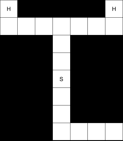
“In this exercise, you are asked to extend dynamic programming to an environment with a single hidden state variable. The environment is a maze with a designated start marked “S”, and two possible goal states, both marked “H”.
“What the agent does not know is which of the two goal states provides a positive reward. One will give +100, whereas the other will give -100. There is a .5 probability that either of those situations is true. The cost of moving is -1; the agent can only move into the four directions north, south, east, and west. Once a state labeled “H” has been reached, the play is over.”
So far, so good.
“(a) Implement a value iteration algorithm for this scenario. Have your implementation compute the value of the starting state. What is the optimal policy?”
The optimal policy here depends on whether we assume the agent must move. If the agent is allowed to remain stationary, then the value of the starting state is 0, because the optimal policy is to stay put.
Calculating the expected reward from reaching state “H” is straightforward. The expected reward is 0, because there’s a 50% chance of a +100 reward, but also a 50% chance of a -100 reward.
0.5 * (+100) + 0.5 * (-100) = 50 + (-50) = 0
Once we establish that, the optimal policy is intuitive. There is no positive reward for reaching any state, but there is a cost to moving to any state. Don’t incur a cost if there’s no possible reward.
The optimal policy changes, however, if the rules state that we must move. In that case, we want to end the game as quickly as possible.
Under this set of rules, the value function decreases as we approach either “H”. The intuition is that the game has no benefits, only costs, so we want to end the game as quickly as possible. From a policy perspective, we want to follow the gradient toward higher values, so if we start at “S”, we wind up trending toward “H”.
“(b) Modify your value algorithm to accommodate a probabilistic motion model: with 0.9 chance the agent moves as desired; with 0.1 chance it will select any of the other three directions at random. Run your value iteration algorithm again, and compute both the value of the starting state, and the optimal policy.”
Once again, the optimal policy depends on whether we can remain stationary. If we can remain stationary, then the value of all cells is 0, and the optimal policy is to stay put. The uncertainty in motion that has just been introduced does not affect the policy, because there’s still no reward for moving anywhere.
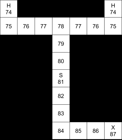
If, however, we are required to move, calculating the policy becomes more complex. At this point we really need a computer to calculate the value function, because we have to iterate over all the cells on the map until values converge. For each cell, we have to look at each action and sum the 90% probability that the action will execute properly, and the 10% probability that the action will misfire randomly. Then we pick the highest-value action. Once we do this for every cell, we repeat the cycle over all the cells again, and we keep doing this until the values stabilize.
The first pass in the iteration sets all cells to 0. Depending on which direction we iterate from, the next step might look like this:
Nonetheless, even without a computer, it seems pretty clear that the optimal policy is still for our agent to stay put in the start cell. Without any information about which “H” is heaven and which is hell, there’s no ultimate reward for going anywhere.
“(c) Now suppose the location labeled X contains a sign that informs the agent of the correct assignment of rewards to the two states labeled “H”. How does this affect optimal policy?”
Without computing the policy, it seems likely that the optimal policy will involve going to the sign, identifying heaven and hell on the map, and then proceeding to heaven.
This policy seems qualitatively clear because of the relatively high payoff for reaching heaven (+100), the relatively low cost of motion (-1), the relatively high probability of the motion executing accurately (0.9), and the relatively small size of the map (distance from S to X to H = 19).
It’s easy to imagine tweaking these parameters such that it’s no longer so obvious that it makes sense to go find the sign. With different parameters, it might still make sense to stay put at S.
“(d) How can you modify your value iteration algorithm to find the optimal policy? Be concise. State any modifications to the space over which the value function is defined.”
Basically, we need to figure out the value of reaching the sign. There are essentially two value functions: the value function when we cannot observe the state, and the value function when we can.
Another way to put this is that going to the sign is like taking a measurement with a sensor. We have prior beliefs about the state of the world before we reach the sign, and then posterior beliefs once we get the information from the sign. Once we transition from prior to posterior beliefs, we will need to recalculate our value function.
An important point here is that this game assumes the sign is 100% certain, which makes the model fully observable. That’s not the case with normal sensors, which is why real robots have to deal with partially observable Markov decision processes (POMDPs).
“(e) Implement your modification, and compute both the value of the starting state and the optimal policy.”
Again, we’d need to write code to actually implement this, but the general idea is to have two value functions. The value of X will be dependent on the posterior value function (the value function that we can calculate once we know which is heaven and which is hell). Then we use that value of X to calculate our prior distribution.
For example, here are the value functions, assuming perfect motion:
The posterior value function, after reading the sign at “X”.The prior value function, before reading the sign at “X”.
The discussion centered around how to generate training data for machine learning, and I spoke specifically about simulated data for self-driving cars.
Tomorrow (Sunday), I will be speaking on the AI-AI-Oh! panel, about training data for machine learning. You should come!
We are going head-to-head for audience size with the CTO of Walmart, who is presenting about shopping in the conference room next door, and I want to win.
This is my first time at SXSW and goodness is it an overwhelming event. There must be thousands of events over 10 days, and they’re always adding new topics. Somehow I missed that Malcolm Gladwell is interviewing Chris Urmson right now!
I present tomorrow, and I’ll be here for a few more days after that, so let me know if you’d like to say hello!
It’s a terrific summary of the current state of deep learning research, reasons why DeepRL is not yet living up to its hype, and hope for the future. It’s written by Alexander Irpan, who works on RL at Google Brain.
“For purely getting good performance, deep RL’s track record isn’t that great, because it consistently gets beaten by other methods.”
There is a lot of interest in using DeepRL for self-driving cars. While this is a super-exciting opportunity in theory, in practice DeepRL has not been effective.
“I tried to think of real-world, productionized uses of deep RL…The way I see it, either deep RL is still a research topic that isn’t robust enough for widespread use, or it’s usable and the people who’ve gotten it to work aren’t publicizing it. I think the former is more likely.”
A big challenge for RL generally, and particularly when it comes to self-driving cars, is the design of a reward function. It’s not clear what the reward function for driving a car would be. And, as Irpan makes clear, unless the reward function is designed near perfectly, the learning agent is going to find all sorts of disastrous shortcuts to maximize the learning function at the expense of violating the implicit rules of the game.
“A friend is training a simulated robot arm to reach towards a point above a table. It turns out the point was defined with respect to the table, and the table wasn’t anchored to anything. The policy learned to slam the table really hard, making the table fall over, which moved the target point too. The target point just so happened to fall next to the end of the arm.”
Irpan is hopeful about the future of RL for practical problems, but cautiously so. Definitely worth a read.
Next Wednesday, March 7, I’ll be holding a workshop on Deep Learning for Autonomous Vehicles as part of the Automotive Tech.AD conference in Berlin. My colleague Aaron Brown and I will walk participants through how to build and train basic convolutional neural networks for traffic sign recognition.
If you work in the automotive industry and have read a lot about deep neural networks, but have never built them yourself, this is the workshop for you. You’ll get hands-on experience setting up and training your own classification networks.
TensorFlow is Google’s library for deep learning, and one of the most popular tools for building and training deep neural networks. In the previous lesson, MiniFlow, students build their own miniature versions of a deep learning library. But for real deep learning work, an industry-standard library like TensorFlow is essential.
Students learn the differences between regression and classification problems. Then they to build a logistic classifier in TensorFlow. Finally, students use fundamental techniques like activation functions, one-hot encoding, and cross-entropy loss to train feedforward networks.
Most of these topics are already familiar to students from the previous “Introduction to Neural Networks” and “MiniFlow” lessons, but implementing them in TensorFlow is a whole new animal. This lesson provides lots of quizzes and solutions demonstrating how to do that.
Towards the end of the lesson, students walk through a quick tutorial on using GPU-enabled AWS EC2 instances to train deep neural networks. Thank you to our friends at AWS Educate for providing free credits to Udacity students to use for training neural networks!
Deep learning has been around for a long time, but it has only really taken off in the last five years because of the ability to use GPUs to dramatically accelerate the training of neural networks. Students who have their own high-performance GPUs are able to experience this acceleration locally. But many students do not own their own GPUs, and AWS EC2 instances are a cloud tool for achieving the same results from anywhere.
The lesson closes with a lab in which students use TensorFlow to perform the classic deep learning exercise of classifying characters: ‘A’, ‘B’, ‘C’ and so on.
The network and the paper in question were clearly designed for autonomous driving, which Apple has been working on, more or less in secret, for years.
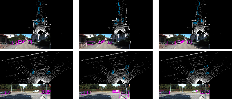
The network in question — VoxelNet — has been trained to perform object detection on lidar point clouds. This isn’t a huge leap from object detection on images, which has been a topic of deep learning research for several years, but it is a new frontier in deep learning for autonomous vehicles. Kudos to Apple for publishing their results.
VoxelNet (by Apple), draws heavily on two previous efforts at applying deep learning to lidar point clouds, both by Baidu-affiliated researchers. Since the three papers kind of work as a trio, I did a quick scan of them together.
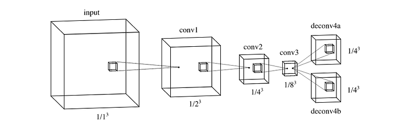
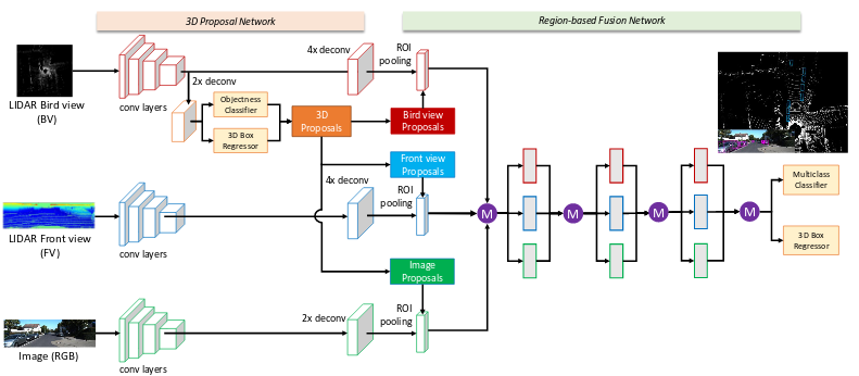
A team of Tsinghua and Baidu researchers developed Multi-View 3D (MV3D) networks, which combine lidar and camera images in a complex neural network pipeline.
In contrast to Li’s solo work, which constructs voxels out of the lidar point cloud, MV3D simply takes two separate 2D views of the point cloud: one from the front and one from the top (birds’ eye). MV3D also uses the 2D camera image associated with each lidar scan.
That provides three separate 2D images (lidar front view, lidar top view, camera front view).
MV3D uses each view to create a bounding box in two-dimensions. Birds-eye view lidar created a bounding box parallel to the ground, whereas front-view lidar and camera view each create a 2D bounding box perpendicular to the ground. Combining these 2D bounding boxes creates a 3D bounding box to draw around the vehicle.
At the end of the network, MV3D employs something called “deep fusion” to combine output from each of the three neural network pipelines (one associated with each view). I’ll be honest — I don’t really understand how “deep fusion” works, so leave me a note in the comments if you can follow what they’re doing.
The results are a classification of the object and a bounding box around it.
That brings us to VoxelNet, from Apple, which got so much press recently.
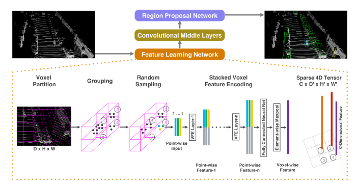
VoxelNet has three components, in order:
Feature Learning Network
Convolutional Middle Layers
Region Proposal Network
The Feature Learning Network seems to be the main “contribution to knowledge”, as the scholars say.
It seems that what this network does is start with a semi-random sample of points from within “interesting” (my word, not theirs) voxels. This sample of points gets run through a fully-connected (not fully-convolutional) network. This network learns point-wise features which are relevant to the voxel from which the points came.
The network, in fact, uses these point-wise features to develop voxel-wise features that describe each of the “interesting” voxels. I’m oversimplifying wildly, but think of this as learning features that describe each voxel and are relevant to classifying the part of the vehicle that is in that voxel. So a voxel might have features like “black”, “rubber”, and “treads”, and so you could guess that the voxel captures part of a tire. Of course, the real features won’t necessarily be intelligible by humans, but that’s the idea.
These voxel-wise features can then get pumped through the Convolutional Middle Layers and finally through the Region Proposal Network and, voila, out come bounding boxes and classifications.
One of the most impressive parts of this line of research is just how new it is. The two Baidu papers were both first published online a year ago, and only made it into conferences in the last six months. The Apple paper only just appeared online in the last couple of weeks.
It’s an exciting time to be building deep neural networks for autonomous vehicles.
Exploring how to build a Self-Driving Car, step-by-step with Udacity!
Editor’s note: David Silver (Program Lead for Udacity’s Self-Driving Car Engineer Nanodegree program), continues his mission to write a new post for each of the 67 lessons currently in the program. We check in with him today as he introduces us to Lesson 5!
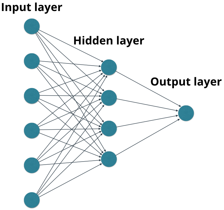
The lesson starts with a fairly basic, feedforward neural network, with just a few layers. Students learn to build the connections between the artificial neurons and implement forward propagation to move calculations through the network.
A feedforward network.
The real mind-bend comes in the “Linear Transform” concept, where we go from working with individual neurons to working with layers of neurons. Working with layers allows us to dramatically accelerate the calculations of the networks, because we can use matrix operations and their associated optimizations to represent the layers. Sometimes this is called vectorization, and it’s a key to why deep learning has become so successful.
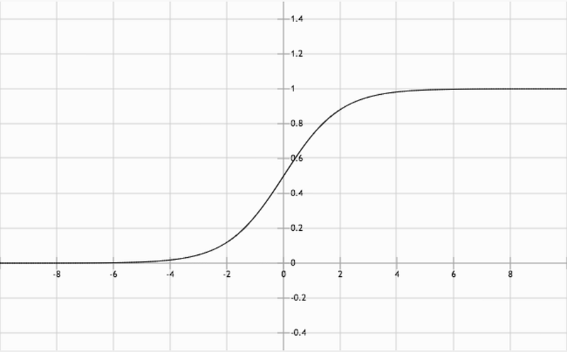
Once students implement layers in MiniFlow, they learn about a particular activation function: the sigmoid function. Activation functions define the extent to which each neuron is “on” or “off”. Sophisticated activation functions, like the sigmoid function, don’t have to be all the way “on” or “off”. They can hold a value somewhere along the activation function, between 0 and 1.
The sigmoid function.
The next step is to train the network to better classify our data. For example, if we want the network to recognize handwriting, we need to adjust the weight associated with each neuron in order to achieve the correct classification. Students implement an optimization technique called gradient descent to determine how to adjust the weights of the network.
Gradient descent, or finding the lowest point on the curve.
Finally, students implement backpropagation to relay those weight adjustments backwards through the networks, from finish to start. If we do this thousands of times, hopefully we’ll wind up with a trained, accurate network.
And once students have finished this lesson, they have their own Python library they can use to build as many neural networks as they want!
Editor’s note: On November 1st of this year, David Silver (Program Lead for Udacity’s Self-Driving Car Engineer Nanodegree program) made a pledge to write a new post for each of the 67 lessons currently in the program. We check in with him today as he introduces us to Lesson 4!
This is a fast lesson that covers the basic mechanics of machine learning and how neural networks operate. We save a lot of the details for later lessons.
My colleague Luis Serrano starts with a quick overview of how regression and gradient descent work. These are foundational machine learning concepts that almost any machine learning tool builds from.
Luis is great at this stuff. I love Mt. Errorest.
Moving on from these lessons, Luis goes deeper into the distinction between linear and logistic regression and then explores how these concepts can reveal the principles behind a basic neural network.
See the slash between the red and green colors there? If you ever meet Luis in person, ask him to sing you the forward-slash-backward-slash alphabet song. It’s amazing.
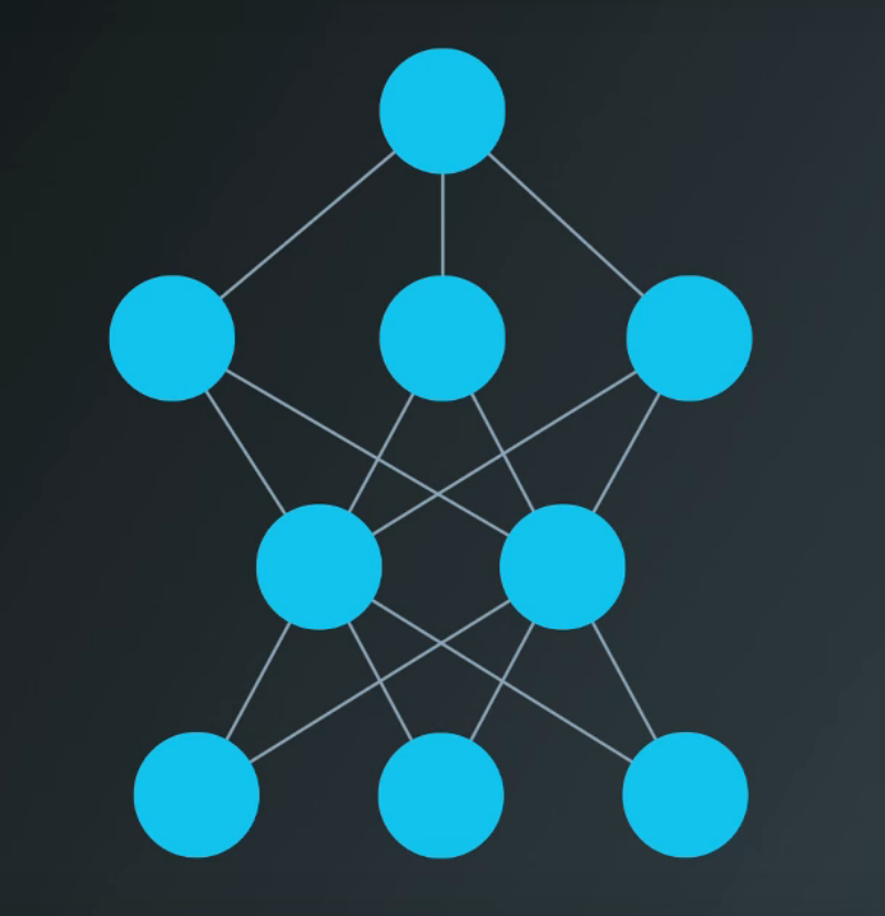
From here we introduce perceptrons, which historically were the precursor to the “artificial neurons” that make up a neural network.
As we string together lots of these perceptrons, or “artificial neurons”, my colleague Mat Leonard shows that we can take advantage of a process called backpropagation, that helps train the network to perform a task.
And that’s basically what a neural network is: a machine learning tool built from layers of artificial neurons, which takes an input and produces an output, trained via backpropagation.
This lesson has 23 concepts (pages), so there’s a lot more to it than the 3 videos I posted here. If some of this looks confusing, don’t worry! There’s a lot more detail in the lesson, as well as lots of quizzes to help make sure you get it.